The Primal-Dual approach for TV inpainting
The primal-dual algorithm was introduced by A. Chambolle and T. Pock in : a first-order primal-dual algorithm for convex problems with applications to imaging, Journal of Mathematical Imaging and Vision, Volume 40, Number 1 (2011), 120-145. In the following, we review this algorithm and implement it for TV inpainting.
Let's consider the general optimisation problem:
\[ \begin{equation*} \min_{x\in \mathbb{R}^N} F(Ax) + G(x) , \end{equation*} \]
where \(A \in \mathbb{R}^{m\times N}\) and \(F: \mathbb{R}^m \to (-\infty, +\infty]\) and \(G: \mathbb{R}^N: (-\infty, +\infty]\) are extended real-valued lower semi-continuous covnex functions. The associated saddle-point problem is
\[ \begin{equation*} \min_{x\in\mathbb{R}^N} \max_{v\in\mathbb{R}^m} G(x) + \langle Ax, v \rangle - F^*(v) . \end{equation*} \]
By taking the first variations of this, we see that \(x^\star\) and \(v^\star\) are solutions to this problem if and only if
\[ \begin{equation*} Ax^\star \in \partial F^*(v^\star) \qquad \textrm{and}\quad -A^T v^\star \in \partial G(x^\star) . \end{equation*} \]
We can rewrite this as
\[ \begin{equation*} \begin{aligned} v^\star + \delta Ax^\star \in v^\star + \delta \partial F^*(v^\star) &\quad \Longleftrightarrow \quad v^\star = \mathrm{Prox}_{\delta F^*}(v^\star + \delta Ax^\star) \\ x^\star - \tau A^T v^\star \in x^\star + \tau \partial G(x^\star) &\quad \Longleftrightarrow \quad x^\star = \mathrm{Prox}_{\tau G}(x^\star - \tau A^T v^\star) . \end{aligned} \end{equation*} \]
Here, given a function \(H\), its proximity operator is defined by
\[ \begin{equation*} \mathrm{Prox}_{\gamma H}(y) = \arg\min_{x} \gamma H(x) + \tfrac{1}{2} \|x-y\|^2 . \end{equation*} \]
This characerisation of \(x^\star\) and \(v^\star\) suggests ths following iterative scheme: introduce an additional variable \(\bar{x}\) and computing the following iterations, for \(\theta \in [0, 1]\), \(\delta, \tau > 0\) such that \(\delta\tau \|A\|^2 < 1\)
\[ \begin{equation*} \begin{aligned} v_{k+1} &= \mathrm{Prox}_{\delta F^*}(v_k + \delta A \bar{x}_k) \\ x_{k+1} &= \mathrm{Prox}_{\tau G}(x_k - \tau A^T v_{k+1}) \\ \bar{x}_{k+1} &= x_{k+1} + \theta (x_{k+1} - x_k) , \end{aligned} \end{equation*} \]
which is the primal-dual algorithm.
So, if \(\mathrm{Prox}_{\delta F^*}\) and \(\mathrm{Prox}_{\tau G}\) are easy to evaluate, then the primal-dual algorithm is an efficient way to solving our optimisation problem.We remark that by Moreau's identity, the proximal mapping associated with \(F^*\) can be computed from the proximal mapping of \(F\) by
\[ \begin{equation*} x = \mathrm{Prox}_{\delta F^*}(x) + \tau \mathrm{Prox}_{\delta F/delta}(x/\delta) . \end{equation*} \]
Let us apply the primal-dual algorithm to total variation inpainting
\[ \begin{equation*} \min_{f} \mathrm{TV}(f) \quad \textrm{subject to} \quad f_{\Omega \setminus D} = g_{\Omega \setminus D} . \end{equation*} \]
Here, \(\Omega\) is our image domain, \(D\) is the inpainting domain, and \(g\) is the original image. To apply the primal-dual algorithm, we shall let
\[ \begin{equation*} F(f) = \|f\|_1 ,\quad G(f) = \iota_{ \{ f_{\Omega \setminus D} = g_{\Omega \setminus D} \} }(f) \quad \textrm{and} \quad A = \nabla . \end{equation*} \]
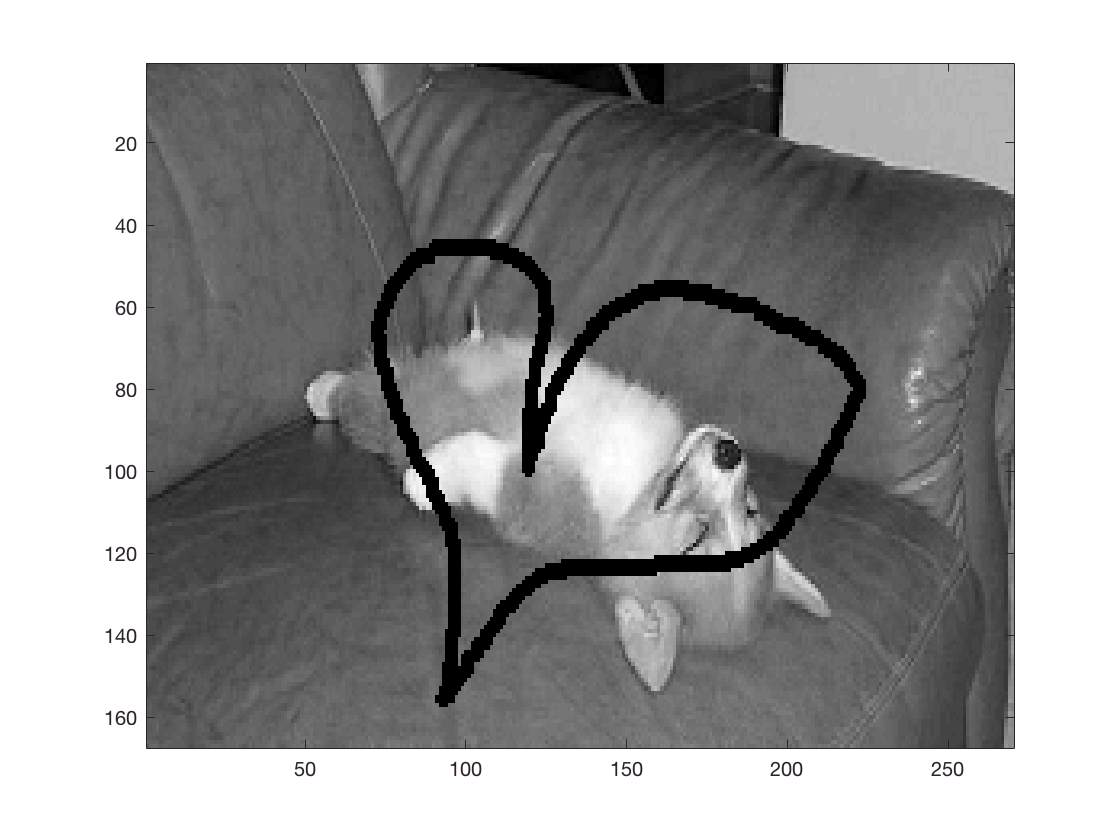
First, load the test image:
image = 'sleeping_dog_des2.PNG';

gcolor=imread(image);
g = double(rgb2gray(gcolor));
g= g/max(g(:));

%
% a=5;
% g =zeros(200);
% g(30:170,30:170)=1;
% g(:, 100-a:100+a)=0.5;

[m,n]=size(g);

figure, imagesc(g), colormap(gray)
 |
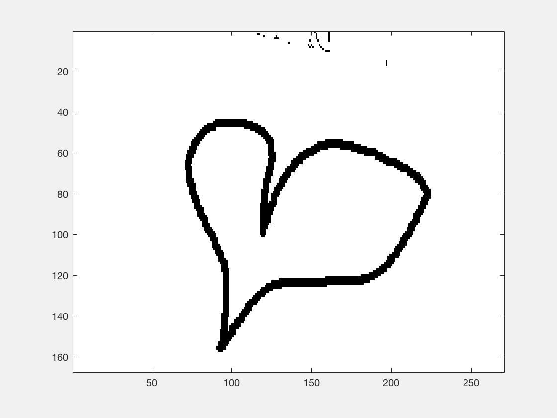
Define the inpainting domain:
y=(g==0);%(abs(g-0.5)<0.2);
mask= 1-y; %mask equals 0 on D and equals 1 on elsewhere.

figure(2)
imagesc(mask); colormap('gray');
 |
Define the proximal operators. One can show that
\[ \begin{equation*} \mathrm{Prox}_{G}(z)_j = \left\{ \begin{aligned} g_j &: j \notin D \\ z_j &: j \in D \end{aligned} \right. \quad\textrm{and}\quad \mathrm{Prox}_{\delta F}(z)_j = \left\{ \begin{aligned} \mathrm{sign}(z_j)(|z_j| - \delta) &: |z_j| \geq \delta \\ 0 &: o.w. \end{aligned} \right. \end{equation*} \]
Prox_G = @(z) z + mask.*g-mask.*z;

abs2 = @(z) repmat( sqrt(abs(z(:,1:n)).^2 +abs(z(:,1+n:end)).^2), 1,2);
sign2 = @(z) [real(sign(z(:,1:n)+1i*z(:,1+n:end))), imag(sign(z(:,1:n)+1i*z(:,1+n:end)))];
Prox_F = @(sigma, z) sign2(z).*(abs2(z)-sigma).*(abs2(z)>=sigma) ;
Prox_FS = @(sigma,z) z-sigma*Prox_F(1/sigma, z/sigma);
Define the gradient operator and its adjoint (we write \(A(f) = [\partial_1 f, \partial_2 f]\)):
A = @(f) [f - circshift(f,1,1) ,f - circshift(f,1,2)];
AS = @(f) (f(:, 1:n)- circshift(f(:, 1:n),-1,1) ) ...
            +(f(:,n+1:end)-circshift(f(:,n+1:end),-1,2));
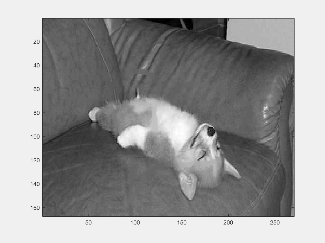
Define the primal-dual iterations (here, we stop when we reach a maximum number of iterations, but one can also use the 'primal dual gap’ as a stopping criterion, i.e. stop when the difference between the primal and dual problems is sufficiently small):
x =zeros(m,n);
xi = A(zeros(m,n));
xbar = zeros(m,n);

maxit = 2000;
sigma = 2; tau=.95/16/sigma; theta=1;

for it = 1:maxit
    xi = Prox_FS(sigma, xi +sigma*A(xbar));
    xold = x;
    x = Prox_G(x-tau*AS(xi));
    xbar = x+theta*(x-xold);
end
Display the output:
 |
Exercise
Use the Primal-Dual approach to solve
The total variation denoising problem, for a given noisy image
\[ \begin{equation*} \min_{f} \mathrm{TV}(f) + \frac{\lambda}{2}\|f-g\|^2 . \end{equation*} \]
\(\ell_1\) regularisation problem, such as
\[ \begin{equation*} \min_{\alpha} \|\alpha_1\|_1 + \frac{\lambda}{2}\|FW^{-1}\alpha-y\|^2 , \end{equation*} \]
where \(F\) is a subsampled Fourier transform and \(W\) is a wavelet transform.